Visualizing Cliques amongst your Professional LinkedIn Connections
Follow @debarghya_dasUnsurprisingly, the information you put up on your LinkedIn says a lot about your professional past and aspirations. I thought it’d be cool to visualize not just my connections who are similar to me, but be able to figure out clusters and relationships amongst my connections.
We do this using a tf-idf weighted bag of words model with a t-SNE visualization.
Getting the Data
Getting brief snippets of all your connections
I scraped all my data off LinkedIn. On your LinkedIn, you can find a (shortened) list of your connections at Connections > Keep in Touch. I had to do a bit of programmatic scrolling to get them all. Running this Javascript from your browser’s console essentially tells it to scroll 100 pixels further down the furthest scroll position of the page’s window every 100 milliseconds.
setInterval(
  function() {
    $(window).scrollTop(
      $(window).scrollTop() + 100
    );
  },
  100
)
Every scroll event to the bottom triggers an API call to load more of your connections and in a few seconds to a few minutes, depending on how many connections you have, all of them will have loaded. At this point, you can do something super low-tech like typing in document.documentElement.outerHTML to get all the HTML contents of the page. I copied all this content into a file on my local computer, and use a Python package called BeautifulSoup along with lxml for quick HTML parsing. A quick examination of the HTML will reveal what CSS selector grabs the data you need - a name, a link to the person’s profile, a designation, a company and a location (though some of the fields are optional). BeautifulSoup provides a great API to use selectors and soon I had a list of a little over a 1000 connections and some brief details.
Scraping your connections’ profiles
Getting the details from your connections are a little harder. For the length and scope of what I was trying to do, I thought it would be a. boring and b. overkill to try and extract the entities associated which each profile (colleges, companies, etc). Instead, I thought it’d be enough to just extract all the text associated with a a person’s profile.
The library I use for most scraping jobs is requests. Along with BeautifulSoup, the two are a deadly internet mining combination. Initially I ran into several problems with scraping https with requests on Python 2.7, so I had to switch my Python virtualenv (if you don’t use virtual environemnts yet, this is a good guide). The format of a connection’s profile is https://www.linkedin.com/profile/view?trk=contacts-contacts-list-contact_name-0&id={id}. It turned out the link from the connections page executes a redirect to this URL, but I extracted the ID with a regex from the previous link. That wasn’t it. This will by default scrape a LinkedIn login page. To get the actual contents, you can copy over your LinkedIn cookie from Chrome (you’ll find this information in the request headers every time you load a page on LinkedIn). Another slightly easier way to get cookies is with a nifty little Chrome extension called EditThisCookie. The requests API allows you to specify request headers as a Python dict along with your .get() request. That did the magic.
The CSS selectors of a connection’s page were also a tad trickier to nail down. Thankfully, BeautifulSoup provides a lovely API to apply regular expressions in your selectors. This was the selector that I used: ^background-.*[^(content)|(section)]. This gives us all the background information of a connection without grabbing the outer divs to avoid getting duplicate text. It generalized well to the 7 or 8 sections LinkedIn profiles could optionally contain. It’s also important to parse out disruptive <script> and <iframe> tags from the results - LinkedIn profiles seemed to contain a lot of them. With what’s left, the .strings property on the BeautifulSoup sections gave me all the information needed.
Bag of Words
Bag of Words is one of the earliest and simplest language models. It was first introduced in Distributional Structure, Zellig Harris, 1954. The idea is that one can represent a piece of text as a discrete distribution of its words (on the global vocabulary of the corpus).
####Example Consider the two sentences.
sen_1 = 'Nawazuddin is a deep learner.'
sen_2 = 'See, his deep learner can see far.'
Let’s assume this is the our entire corpus, or set of documents we know about. The vocabulary we are aquainted with is
{
  'nawazuddin',
  'is',
  'a',
  'deep',
  'learner',
  'his',
  'can',
  'see',
  'far'
}
The bag-of-words representence of the two sentences would then be
sen_1_bow = [1, 1, 1, 1, 1, 0, 0, 0, 0]
sen_2_bow = [0, 0, 0, 1, 1, 1, 1, 2, 1]
In Real Life Data
In large quantities of real world data, the vocabulary space can expand upto 200,000 and vectors for each document are usually sparse. The way one would typically estimate similarity between two documents is computing the cosine similarity between the vectors. Identical distributions have a similarity of 1 and distributions where there are no words in common have similarities are 0.
The assumption in the bag of words model is that the ordering of words in a sentence or a document are irrelevant. You’ll notice that two documents with the same words will have the same representation irregardless of whether their actual arrangement in the text changes their meaning. For example The New University of York and New York University would have a high similarity despite having absolutely no semantic similarity.
Another crucial disadvantage is that the model asserts equal importance to all words in the vocabulary. Two documents may have similar number of pronouns, prepositions and articles but those similarities are not as important as, say, proper nouns like college names and institutions. However, there are not so difficult ways to get around this we’ll explore later.
Other issues with bag of words include the fact that words can half multiple meanings in multiple contexts (My sleep was deep, The pool was deep), negatory words can reverse semantic meaning without affecting the distribution much (I'm not a good person, I'm a good person), groups of multiple words can have semantic meaning together and different meaning separately (new york, new things in york) and more. There are far better models than bag of words such as word2vec and A Neural Probabilistic Language Model, Bengio et al, 2003 and more.
Tf-idf Weighted Bag of Words
Tf-idf, or term frequency - inverse document frequency, is a statistic to determine how important a word is in a corpus. It’s the multiple of the term frequency - the number of times a word occurs in a document and the inverse of the document frequency - the number of documents this word occurs in. Tfidf weightings automatically make stop words like prepositions, pronouns and articles less relevant in the vector space bag of words representation of a document and makes specific words like proper nouns more heavily weighted.
t-distributed Stochastic Neighbor Embedding (t-SNE)
Ever since I read this post by Andrej Karpathy, I’ve been wanting to play around with t-SNE. I couldn’t agree more with Andrej:
t-SNE comes across as one that has a pleasing, intuitive formulation, simple gradient and nice properties.
t-SNE is one of the many ways (others include PCA, Kernel PCA, Isomap, LLE, Autoencoders, etc) to reduce data in higher dimensional spaces onto lower dimensions. Uses of this can range from reducing the number of significant dimensions of the data and thereby reducing the number of random variables under consideration in a given learning algorithm, or just visualization. t-SNE’s properties make it ideal for visualization, and was first introduced in Visualizing Data using t-SNE, van der Maaten and Hinton, 2008 and an awesome explanation is available from van der Maatens’ video here.
The formulation for t-SNE is quite intuitive - we set up metrics for distance in both the higher dimensional space and the lower dimensional space and then we minimize a formulation of the differences between these distances in the two spaces. The formulation of t-SNE is based on KL-divergence, and the significance of this is that it keeps close points in the high dimensional space close in the lower dimensional space while allowing furher points to move around freely. This makes for a good visualization.
You can find multiple implementations of t-SNE on van der Maaten’s site, but the most convenient one for me was built into scikit-learn. Having watched the video, it doesn’t seem terribly difficult to implement the algorithm from scratch as good practice too.
The original implementation of t-SNE runs in \O(n^2)\ which is quite slow on large amounts of data (although okay for this particular project). It’s accelerated to \O(nlogn)\ using quad-trees in what’s known as the Barnes-Hut t-SNE approximation.
Visualization
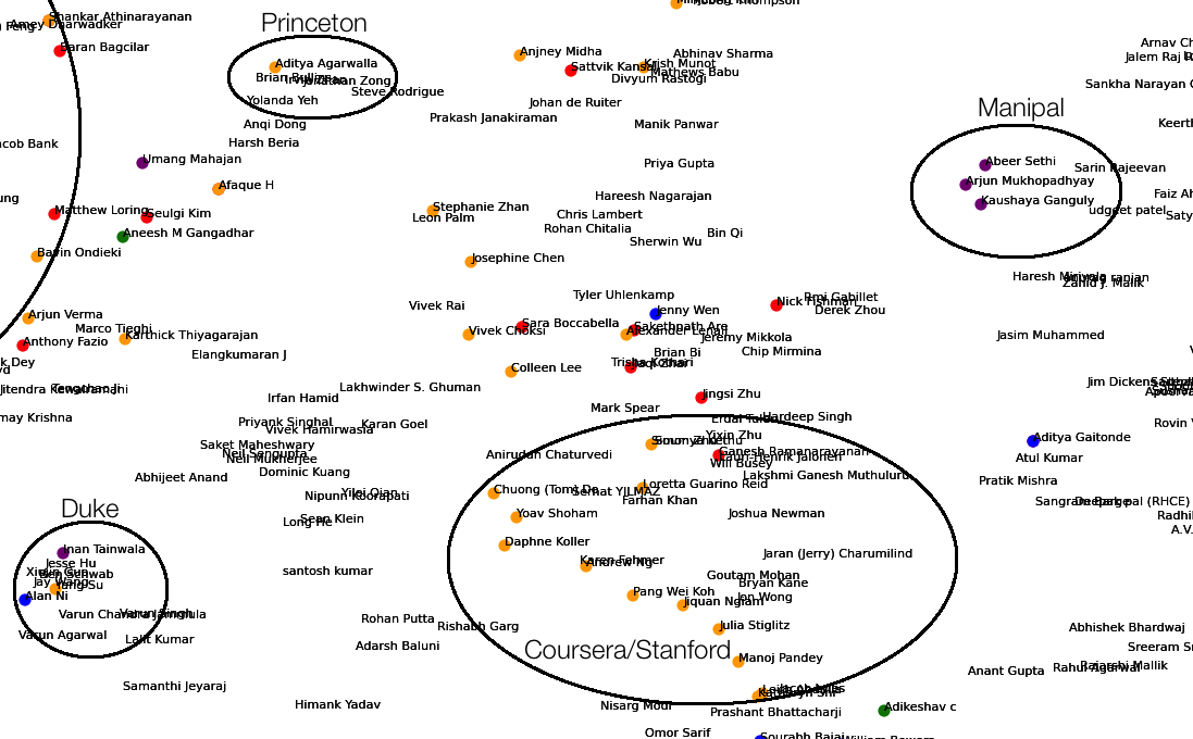
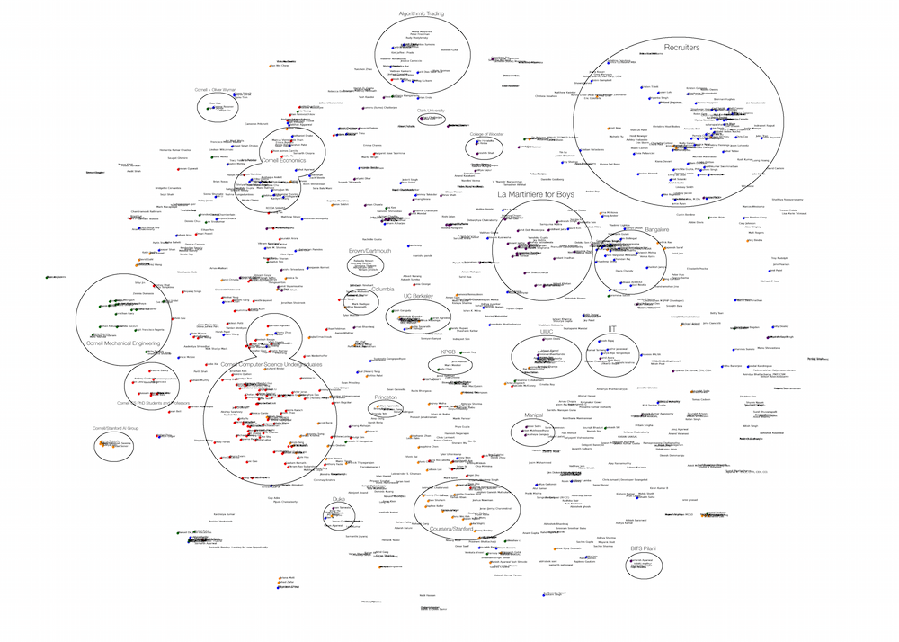
The results I expected from the visualization were to see people from similar colleges, companies, industries and majors cluster together and disparate ones be further apart. Indeed, the tf-idf bag of words with t-SNE worked well. Some of the many groups I noticed were
- A huge cluster of people from the same college
- Cornell
- Brown/Dartmouth (for some reason, these were conflated into one)
- Columbia
- UC Berkeley
- Stanford
- Princeton
- Clark
- College of Wooster
- Manipal
- BITS Pilani
- IIT
- Duke
- UIUC
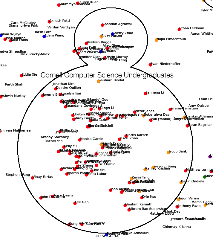
- A dense cluster of people from my undergrad college who were in one major
- Computer Science
- Mechanical Engineering
- Economics
- A large cluster of friends from high school
- Industries/Companies
- Coursera
- KPCB
- Oliver Wyman
- Algorithmic Trading
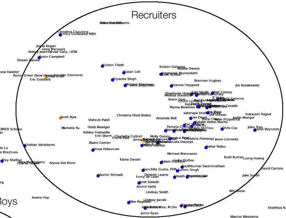
- A gigantic cluster of recruiters (the second biggest one after Cornell)
- Miscellaneous
- There were a group of people who I met and or who live in and around Bangalore
- A ton of floating connections I didn’t remember very well
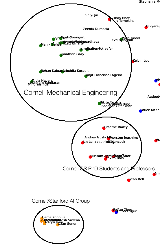
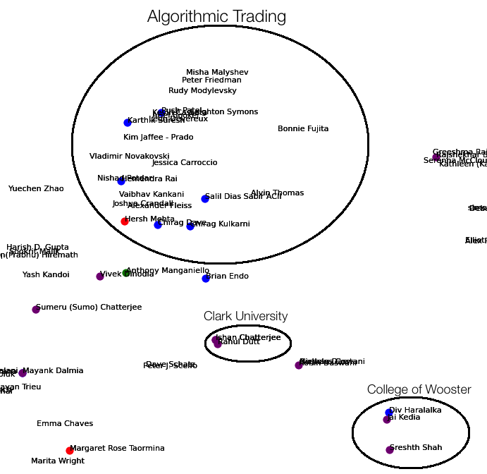
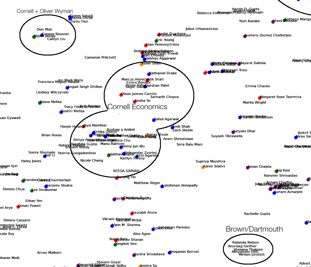
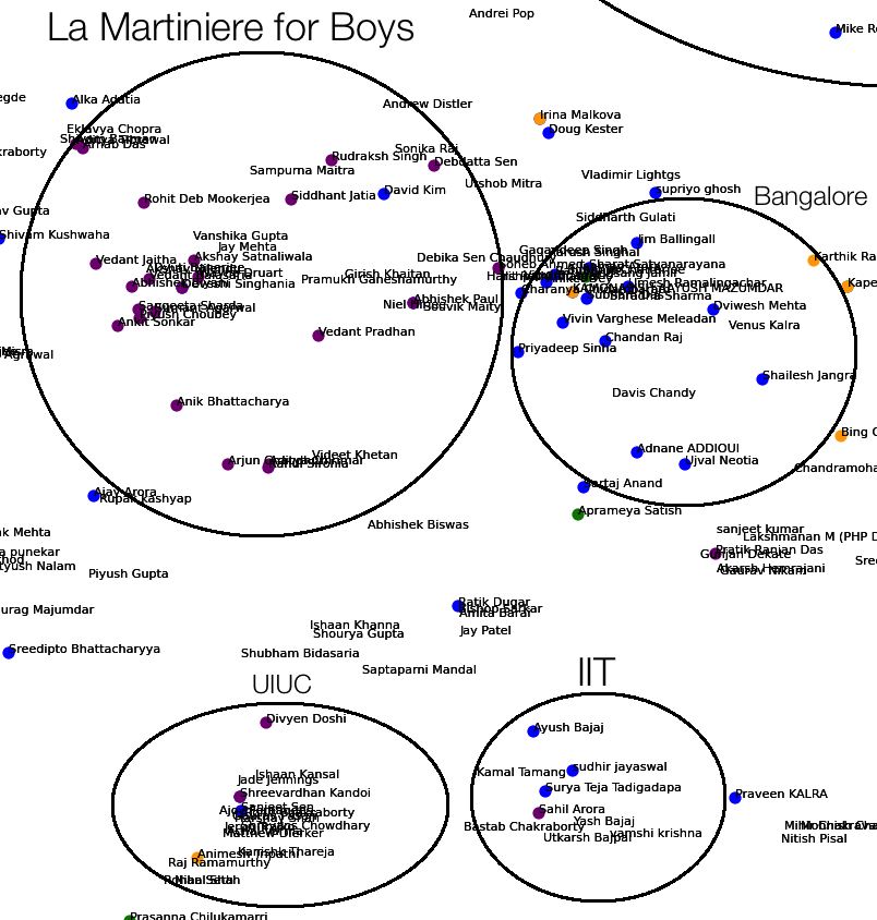
In the images below, the colors represent the following:
- Orange - text contains ‘Computer Science’ and ‘Cornell’
- Blue - text contains Consulting
- Green - text contains ‘Mechanical Engineering’ and ‘Cornell’
- Purple - text contains ‘La Martiniere’
- Yellow - text contains ‘Stanford’
Do note though, that on account of my laziness:
- the colors overwrite each other in the above legend, so if a name has an associated yellow dot on its bottom left, it might also be orange.
- Names with an extremely high similarity are printed on top of each other and aren’t legible.
- I discarded certain connections with too little scraped information (less than 200 characters) on their LinkedIns.
- The unaliased thick black cluster circling are horrible artifacts of my love for Paint (or on OSX, Paintbrush)
A high-res, zoomable, interactive version of the result is available here.
A Low Resolution Overview of the Entire t-SNE embedding
Recruiters
Cornell Computer Science
Cornell Mechanical Engineers, Professors and Stanford/Cornell AI Lab
The Algorithmic Trading, Clark and Wooster Clusters
Cornell Economics majors, Oliver Wyman and Brown/Dartmouth
Bangalore, IIT, La Martiniere and UIUC
Stanford/Coursera, Duke, Manipal and Princeton